Taking Text Embedding and Cosine Similarity for a Test Drive
Introduction
Computational processing of natural languages has always been a difficult task for computers and programmers alike. A given concept has many representations in written text and a given written text can have many different interpretations. In addition, spelling, grammar, and punctuation are not consistent from person to person. Add in metaphors, sarcasm, tone, dialects, jargon, etc. and all compound the problem. The numerous difficulties have created a situation where, until recently, computers have been very poor at working in natural language. Recall the desperation you feel to break out of a company’s chatbot or voice-activated question-answering systems to get to a human being.
One specific problem that, if solved, would have many real-world applications, is the following: If we could confidently determine if two texts have the same conceptual meaning, regardless of the wording that is used, this could have a big impact on search engines. If we could also determine if text had similar or opposite meanings that would strengthen search capabilities even further.
Word embeddings have become a fundamental technique for capturing the semantic meaning of text. An embedding algorithm, when given text to process, returns an array, or more precisely a vector, of numbers that represents the conceptual meaning of the original text. These vectors can be of any length, but we currently see ranges from the low hundreds to over a thousand floating point numbers. Similar concepts will yield similar embedding vectors; the more different the concepts are, the more divergent the embedding vectors will be.
To solve our search problem, we also need a way to measure how similar or different the embeddings are from each other. There are multiple algorithms for this including Euclidean distance and cosine similarity. In this post, we will explore using cosine similarity to assess how different variations in phrasing impact semantic similarity between sentences. We will see how changes like synonyms only slightly alter vector orientations, while sentences having opposite meanings or are completely unrelated cause larger divergence.
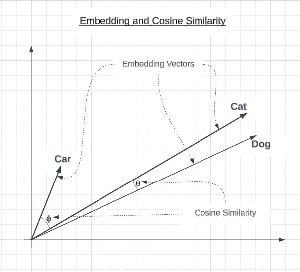
The following is a two-dimensional graph showing sample embedding vectors for car, cat, and dog. The cosine similarity between the cat and dog embedding vectors is fairly small but is larger between cat and car.

While cosine similarity has a range from -1.0 to 1.0, users of the OpenAI embedding API will typically not see values less than 0.4. A thorough explanation of the reasons behind this are beyond the scope of this article, but you can learn more by searching for articles about text embedding pooling.
Obtaining Embeddings and Cosine Similarity
To make this process more tangible, let’s walk through a simple example.
We’ll start with our original phrase: The cat ran quickly.
Using the OpenAI embedding model, “text-embedding-ada-002”, this will produce a 1536-dimensional vector like: (-0.024, …, -0.021)
Now let’s compare it to a similar phrase: The kitten ran quickly. (-0.018, …, -0.018)
To quantify the similarity of these embeddings, we can use the cosine similarity metric which measures the angle between two vectors on a scale from -1 to 1. A score of 1 means identical, 0 is orthogonally different, and -1 is opposite.
The cosine similarity between our original phrase and synonym phrase, “The kitten ran quickly.” is 0.978, indicating the vectors are very close in meaning.
In contrast, an unrelated phrase like “The car was blue,.” with an embedding of (-0.007, …, -0.017) would have a lower cosine similarity to our original phrase, around 0.818.
Example Sentences
To demonstrate the impact of preprocessing on word embeddings, we will use the original phrase and show its abbreviated embedding:
Original
The original sentence we will compare the others to is “The cat ran quickly.” This will be compared against itself and the expected similarities would be 1.0. The original sentence provides the baseline for comparison.
| Sentence | Embedding Vector |
|---|---|
| The cat ran quickly. | (-0.024, …, -0.021) |
Almost Identical Meaning
These sentences have almost the same meaning as the original sentence, with only minor variations. We expect these to have high similarity scores close to 1.0.
| Sentence | Embedding Vector |
|---|---|
| A cat ran quickly. | (-0.025, …, -0.022) |
| The the the The cat ran quickly. | (-0.023, …, -0.019) |
| The CaT RAn Quickly. | (-0.031, …, -0.028) |
| The cat ran, quickly! | (-0.021, …, -0.029) |
| Quickly the cat ran. | (-0.022, …, -0.016) |
| Quickly ran the cat. | (-0.029, …, -0.013) |
Conceptually Close
These sentences are conceptually similar to the original, using synonyms or adding details. We expect moderately high similarity scores.
| Sentence | Embedding Vector |
|---|---|
| The kitten ran quickly. | (-0.018, …, -0.018) |
| The feline sprinted rapidly. | (-0.015, …, -0.019) |
| A kitten dashed swiftly. | (-0.016, …, -0.014) |
| The cat that was brown ran quickly. | (-0.024, …, -0.027) |
| The brown cat ran quickly | (-0.023, …, -0.024) |
| The cat’s paws moved quickly. | (-0.001, …, -0.016) |
| The cat and dog ran quickly. | (-0.021, …, -0.013) |
| The cat ran quickly? | (-0.015, …, -0.026) |
Opposites/Negations
This group of sentences expresses the opposite meaning or negates the original sentence. We expect lower similarity scores.
| Sentence | Embedding Vector |
|---|---|
| The cat did not run quickly. | (-0.017, …, -0.031) |
| The cat walked slowly. | (0.001, …, -0.022) |
| The cat stopped. | (-0.014, …, -0.027) |
Unrelated Concepts
These sentences have no relation in meaning to the original sentence about a cat running. We expect very low similarity scores.
| Sentence | Embedding Vector |
|---|---|
| The automobile drove fast. | (-0.027, …, -0.008) |
| The student studied math. | (0.011, …, -0.04) |
| The tree was green. | (0.004, …, -0.031) |
| The car was blue. | (-0.007, …, -0.017) |
| 3+5=8 | (-0.015, …, -0.034) |
Computing Similarities
Next, we compute the similarity between the embedding of our original sentence and each of the other sentence’s embeddings. The computed similarity between the original sentence’s embeddings and itself is included for reference. The below table shows the similarities, in descending order.
| Category | Sentence | Cosine Similarity |
|---|---|---|
| Original | The cat ran quickly. | 1.0 |
| Almost Identical | A cat ran quickly. | 0.994 |
| Almost Identical | The the the The cat ran quickly. | 0.989 |
| Almost Identical | Quickly the cat ran. | 0.982 |
| Almost Identical | The cat ran, quickly! | 0.979 |
| Conceptually Close | The kitten ran quickly. | 0.978 |
| Conceptually Close | The brown cat ran quickly | 0.975 |
| Conceptually Close | The cat ran quickly? | 0.971 |
| Conceptually Close | The cat that was brown ran quickly. | 0.968 |
| Conceptually Close | The feline sprinted rapidly. | 0.965 |
| Almost Identical | Quickly ran the cat. | 0.965 |
| Conceptually Close | The cat and dog ran quickly. | 0.959 |
| Conceptually Close | A kitten dashed swiftly. | 0.956 |
| Conceptually Close | The cat’s paws moved quickly. | 0.943 |
| Opposites/Negations | The cat did not run quickly. | 0.922 |
| Opposites/Negations | The cat walked slowly. | 0.898 |
| Almost Identical | The CaT RAn Quickly. | 0.89 |
| Opposites/Negations | The cat stopped. | 0.885 |
| Unrelated Concepts | The automobile drove fast. | 0.884 |
| Unrelated Concepts | The car was blue. | 0.818 |
| Unrelated Concepts | The tree was green. | 0.811 |
| Unrelated Concepts | The student studied math. | 0.784 |
| Unrelated Concepts | 3+5=8 | 0.75 |
Analysis
The table below shows the average cosine similarity for each category, sorted in descending order. We can see pretty much what we would expect. The more similar a category of sentences is to the original sentence, the closer to 1.0 its average cosine similarities are.
| Category | Average Cosine Similarity |
|---|---|
| Original | 1.0 |
| Almost Identical | 0.966 |
| Conceptually Close | 0.964 |
| Opposites/Negations | 0.902 |
| Unrelated Concepts | 0.809 |
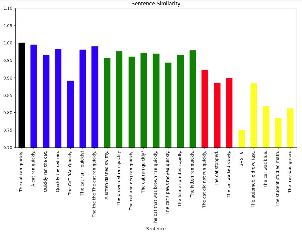
The following bar chart shows each sentence and its similarity. The bar color indicates the category that the sentence belongs to:
- Black for the Original sentence
- Blue for Almost Identical sentences
- Green for Conceptually Close sentences
- Red for Opposites/Negations
- Yellow for Unrelated Concepts

The bar chart visually shows that the categories clustered as expected, with the most similar sentences having cosine similarities closest to 1.0. This validates that the cosine similarity of embeddings captures semantic closeness.
A few possible anomalies we can see from the graph include:
- “The CaT RAn Quickly.” Although it is in the “Almost Identical” category, it is lower than any sentence in the “Conceptually Close” category and is on par with “Opposites/Negations”. Differences in upper and lower case letters can affect the embedding algorithm.
- “The automobile drove fast.” Is particularly high among the other sentences in “Unrelated Concepts” and is closer to the “Opposites/Negatives”. This may be because the word fast implies movement which is also, represented in the original sentence.
- “Quickly ran the cat.” looks like it could be in the “Conceptually Close” or the “Almost Identical” categories. It is not clear why the cosine similarity is marginally smaller than most other “Almost Identical” sentences, but the difference is small.
This was a small experiment but did highlight the potential of using cosine similarity of embedding vectors in language processing tasks. There does appear to be room for improvement through natural language processing techniques, such as lowercasing. However, blindly lowercasing may also negatively impact documents that are rich in acronyms, where capitalization carries meaning. As a result, a more deliberate technique may be needed.
Overall, we can conclude that:
- The similar performance of simple averaging versus a visual categorization shows embeddings numerically capture intuitive human judgments of similarity.
- Synonyms and minor variations like changes in punctuation did not drastically alter the embeddings. This suggests embeddings derive meaning from overall context rather than exact word choice.
- The small gap between “Almost Identical” and “Conceptually Close” categories shows there’s some subjectivity in assessing similarity. The embeddings reflect nuanced gradients of meaning.
Conclusion
Our experiments illustrated how the cosine similarity of embeddings allows us to numerically measure the semantic closeness of text. We saw how small variations may not greatly affect similarity, while more significant changes lead to larger divergence.
Having the ability to map text to concepts, numerically, and then being able to compare the concepts instead of the text strings, unlocks new and improved applications such as:
- Search engines - Match queries to documents based on conceptual relevance, not just keywords
- Chatbots/dialog systems - Interpret user intent and determine appropriate responses
- Voice-activated QA systems - Understand and respond accurately to spoken questions
- Document classifiers - Automatically group texts by topics and meaning
- Sentiment analysis - Identify subtle distinctions in emotional tone beyond keywords
- Text summarization - Determine the degree of shift in meaning between a document and its summary
- Machine translation - Determine the quality of translated text
Potential next steps include trying more diverse text, comparing embedding models, and testing various natural language preprocessing techniques such as the previously mentioned lowercasing of text.
Bob Simonoff is
- A Senior Principal Software Engineer, Blue Yonder Fellow at Blue Yonder.
- A founding member of the OWASP Top 10 for Large Language Model Applications.
- on LinkedIn at www.linkedin.com/in/bob-simonoff
