In the dynamic world of software development, maintaining the integrity of your codebase is paramount. GitHub, a collaborative coding platform, provides a robust toolkit to uphold the quality and security of your projects.

GitHub’s branch protection rules with mandatory status checks stand as a bulwark, ensuring that contributions can only merge into the main branch after passing through quality and security checks.

But hey, you’re still with us! Your interest in CI/CD, DevOps, and the intricate dance of collaboration in the software development world is palpable. Excellent!
Now, let’s dive into the realm of dynamic status checks — a feature not directly supported by GitHub out of the box, but fear not, there are workarounds to achieve this goal.

The Problem

In the branch protection rules of the main branch, configuring the required status checks for a pull request is crucial. Standard checks, such as linting, unit tests, and code coverage, should be typically required for all pull requests.

The following is a workflow example to check the source code changes of an application. The tests are executed in job test after the application got built and deployed. Therefore, job test should be configured as required status check in the branch protection rules.

on:
  pull_request:
    paths:
      - src/**
      - tests/**

jobs:
  build-deploy:
    runs-on: ubuntu-latest
    steps:
      [...]
    
  test:
    needs: build-deploy    
    runs-on: ubuntu-latest
    steps:
      [...]

However, running this workflow is expensive and time-consuming because the application first needs to be built and deployed before the tests can be executed. And the tests themselves can also take quite some time.

Therefore, the test workflow should only be triggered if the source code or the tests themselves have changed. In contrast, unrelated changes such as documentation changes should not trigger code related checks.
This is why the pull_request workflow trigger is limited to changes in directories src and tests, as specified by paths.

But what if the test workflow is not triggered because no files in those directories have changed? Then, the pull request could not be merged because the required status check is not passing, as it was not executed at all.
This is where the problem lies and why we need dynamic status checks that are only required if the relevant files have changed.

Fortunately, there are two workarounds!

Check for relevant Changes

The workaround is to check for the relevant file changes in a job of the workflow itself and execute the actual status check only if the relevant files have changed.
The paths of trigger pull_request are specified in the files input of the tj-actions/changed-files action (or any similar GitHub Action).

This status check doesn’t block the PR from merging if it gets skipped. It only blocks it if it gets executed and fails.

on:
  # Always execute, otherwise GitHub will wait forever for required checks
  pull_request:
    
jobs:
  check-if-relevant:
    runs-on: ubuntu-latest
    outputs:
      is-relevant: ${{ steps.relevant-files-changed.outputs.any_changed }}
    steps:
      # This step is needed by tj-actions/changed-files
      - uses: actions/checkout@v4
        with:
          fetch-depth: 0
      # https://github.com/marketplace/actions/changed-files
      - uses: tj-actions/changed-files@v41.0.1
        id: relevant-files-changed
        with:
          files: |
            src/**
            tests/**
 
  build-deploy:
    needs: check-if-relevant
    if: needs.check-if-relevant.outputs.is-relevant == 'true'
    runs-on: ubuntu-latest
    steps:
      [...]
    
  test:
    needs: build-deploy
    runs-on: ubuntu-latest
    steps:
      [...]

Reusable Workflow as Status Check

The approach works fine for standard workflows, where any job can be configured as status check. However, it doesn’t work for reusable workflows.

In this example the test workflow utilizes reusable workflows for the build and deploy and the test steps.

on:
  pull_request:
    
jobs:
  check-if-relevant:
    runs-on: ubuntu-latest
    outputs:
      is-relevant: ${{ steps.relevant-files-changed.outputs.any_changed }}
    steps:
     [...]
 
  build-deploy:
    needs: check-if-relevant
    if: needs.check-if-relevant.outputs.is-relevant == 'true'
    uses: ./.github/workflows/release.build_deploy.yml
    secrets: inherit    

  test:
    needs: build-deploy
    uses: ./.github/workflows/test.execution.yml
    secrets: inherit
    with:
      app-url: ${{ needs.build-deploy.outputs.app-url }}

The calling job test can’t be set as status check because GitHub ignores its status.

Configuring a job in the called reusable workflow test.execution.yml is not an option either.
If test in the calling workflow would be skipped, the pull request would wait forever for the status check in the reusable workflow as the skipping happens on workflow parent level, not child level.

The workaround is to configure an additional, standard job test-completed that concludes the workflow as status check and fails if the test failed before.
Setting if: always() ensures that the job is always executed, even if the test job failed.

on:
  pull_request:
    
jobs:
  check-if-relevant:
    runs-on: ubuntu-latest
    outputs:
      is-relevant: ${{ steps.relevant-files-changed.outputs.any_changed }}
    steps:
     [...]
 
  build-deploy:
    needs: check-if-relevant
    if: needs.check-if-relevant.outputs.is-relevant == 'true'
    uses: ./.github/workflows/release.build_deploy.yml
    secrets: inherit  

  test:
    needs: build-deploy
    uses: ./.github/workflows/test.execution.yml
    secrets: inherit
    with:
      app-url: ${{ needs.build-deploy.outputs.app-url }}

  test-completed:
    needs: test
    runs-on: 'ubuntu-latest'
    if: always()
    steps:
      - name: Check test job status
        if: needs.test.result == 'failure'
        run: exit 1

Conclude with final Status Check

Another workaround is to add a concluding job like the required-status-check in the following example to all dynamically required workflows.

on:
  pull_request:
    paths:
      - src/**
      - tests/**

jobs:  
  build-deploy:
    runs-on: ubuntu-latest
    steps:
      [...]

  test:
    needs: build-deploy
    runs-on: ubuntu-latest
    steps:
      [...]
    
  required-status-check:
    needs: test
    runs-on: 'ubuntu-latest'
    if: always()
    steps:
      - name: Check workflow status
        if: needs.test.result != 'success'
        run: exit 1

This job would return a failure state if the tests of job test failed.

In the repo settings configure required-status-check as required status check in the branch protection rules of the main branch.
The pull requests get blocked if none of the triggered workflows have implemented the required-status-check job or at least one of them is failing.
It gets unblocked if at least one required-status-check job is implemented and all of them are successful. It’s worth noting that at least one workflow needs to run in any case (e.g. a lint or source formatting check) and can be piggybacked to implement this.

Comparison

Pro relevant Changes Check

• This approach is less complex as the final status check workflow because its fallback workflow has to be kept in mind.
• It’s transparent for a GitHub repo admin what status checks are actually executed by just taking a look at the branch protection rules. Whereas it is not obvious with a general status check such as required-status-check.

Pro final Status Check

• Only those workflows get executed that actually apply to the changed files, because the list of relevant files are declared at the pull_request trigger.
  As a result, the status check overview of the pull request is limited to the relevant checks and no workflow is run unnecessarily.

• The triggers and specific trigger conditions can be configured declaratively.
  Additional triggers besides the pull_request that have to run in any case (even without relevant file changes) can be configured in a clean way. And the files restriction of the pull_request trigger are also declared where you would expect them: in the pull_request trigger.
  
  Declarative config:

  on:
    workflow_dispatch:
    schedule:
      - cron: '0 0 * * 1' # 00:00 on Mondays.
    pull_request:
      paths:
        - package-lock.json
  

  Job config:

  on:
    workflow_dispatch:
    schedule:
      - cron: '0 0 * * 1' # 00:00 on Mondays.
    pull_request:
  
  jobs:    
    check-if-relevant:
      runs-on: ubuntu-latest
      outputs:
      is-relevant: ${{ (github.event_name == 'pull_request' && steps.relevant-files-changed.outputs.any_changed == 'true') || github.event_name != 'pull_request' }}
      steps:
        # https://github.com/marketplace/actions/changed-files
        - uses: tj-actions/changed-files@v41.0.1
          if: github.event_name == 'pull_request'
          id: relevant-files-changed
          with:
            files: package-lock.json
  

Conclusion

GitHub’s branch protection rules with required status checks are a powerful tool to ensure quality and security. They are only missing the ability to configure dynamic status checks that are only required if relevant changed had been committed.

However, we have two workarounds to solve this problem:

1. Check for the relevant file changes in a job of the workflow itself and execute the actual status check only for relevant changes.
2. Add a concluding job to all dynamically required workflows and configure it as required status check.

With GitHub continuously evolving and gathering user feedback, our hope is that the need for such workarounds becomes obsolete.
We look forward to a future where seamless and dynamic status checks align effortlessly with the needs of developers, making these inventive workarounds a thing of the past.

Introduction

Computational processing of natural languages has always been a difficult task for computers and programmers alike. A given concept has many representations in written text and a given written text can have many different interpretations. In addition, spelling, grammar, and punctuation are not consistent from person to person. Add in metaphors, sarcasm, tone, dialects, jargon, etc. and all compound the problem. The numerous difficulties have created a situation where, until recently, computers have been very poor at working in natural language. Recall the desperation you feel to break out of a company’s chatbot or voice-activated question-answering systems to get to a human being.

One specific problem that, if solved, would have many real-world applications, is the following: If we could confidently determine if two texts have the same conceptual meaning, regardless of the wording that is used, this could have a big impact on search engines. If we could also determine if text had similar or opposite meanings that would strengthen search capabilities even further.

Word embeddings have become a fundamental technique for capturing the semantic meaning of text. An embedding algorithm, when given text to process, returns an array, or more precisely a vector, of numbers that represents the conceptual meaning of the original text. These vectors can be of any length, but we currently see ranges from the low hundreds to over a thousand floating point numbers. Similar concepts will yield similar embedding vectors; the more different the concepts are, the more divergent the embedding vectors will be.

To solve our search problem, we also need a way to measure how similar or different the embeddings are from each other. There are multiple algorithms for this including Euclidean distance and cosine similarity. In this post, we will explore using cosine similarity to assess how different variations in phrasing impact semantic similarity between sentences. We will see how changes like synonyms only slightly alter vector orientations, while sentences having opposite meanings or are completely unrelated cause larger divergence.

The following is a two-dimensional graph showing sample embedding vectors for car, cat, and dog. The cosine similarity between the cat and dog embedding vectors is fairly small but is larger between cat and car.

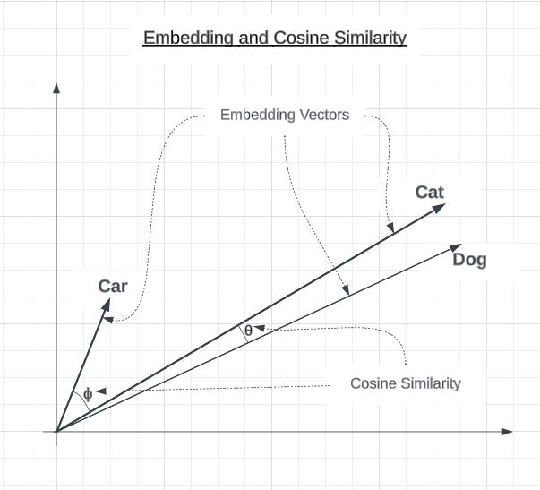
While cosine similarity has a range from -1.0 to 1.0, users of the OpenAI embedding API will typically not see values less than 0.4. A thorough explanation of the reasons behind this are beyond the scope of this article, but you can learn more by searching for articles about text embedding pooling.

Obtaining Embeddings and Cosine Similarity

To make this process more tangible, let’s walk through a simple example.

We’ll start with our original phrase: The cat ran quickly.

Using the OpenAI embedding model, “text-embedding-ada-002”, this will produce a 1536-dimensional vector like: (-0.024, …, -0.021)

Now let’s compare it to a similar phrase: The kitten ran quickly. (-0.018, …, -0.018)

To quantify the similarity of these embeddings, we can use the cosine similarity metric which measures the angle between two vectors on a scale from -1 to 1. A score of 1 means identical, 0 is orthogonally different, and -1 is opposite.

The cosine similarity between our original phrase and synonym phrase, “The kitten ran quickly.” is 0.978, indicating the vectors are very close in meaning.

In contrast, an unrelated phrase like “The car was blue,.” with an embedding of (-0.007, …, -0.017) would have a lower cosine similarity to our original phrase, around 0.818.

Example Sentences

To demonstrate the impact of preprocessing on word embeddings, we will use the original phrase and show its abbreviated embedding:

Original

The original sentence we will compare the others to is “The cat ran quickly.” This will be compared against itself and the expected similarities would be 1.0. The original sentence provides the baseline for comparison.

Almost Identical Meaning

These sentences have almost the same meaning as the original sentence, with only minor variations. We expect these to have high similarity scores close to 1.0.

Conceptually Close

These sentences are conceptually similar to the original, using synonyms or adding details. We expect moderately high similarity scores.

Opposites/Negations

This group of sentences expresses the opposite meaning or negates the original sentence. We expect lower similarity scores.

Unrelated Concepts

These sentences have no relation in meaning to the original sentence about a cat running. We expect very low similarity scores.

Computing Similarities

Next, we compute the similarity between the embedding of our original sentence and each of the other sentence’s embeddings. The computed similarity between the original sentence’s embeddings and itself is included for reference. The below table shows the similarities, in descending order.

Analysis

The table below shows the average cosine similarity for each category, sorted in descending order. We can see pretty much what we would expect. The more similar a category of sentences is to the original sentence, the closer to 1.0 its average cosine similarities are.

The following bar chart shows each sentence and its similarity. The bar color indicates the category that the sentence belongs to:

• Black for the Original sentence
• Blue for Almost Identical sentences
• Green for Conceptually Close sentences
• Red for Opposites/Negations
• Yellow for Unrelated Concepts

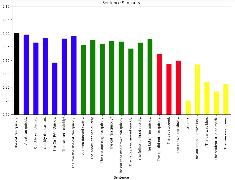
The bar chart visually shows that the categories clustered as expected, with the most similar sentences having cosine similarities closest to 1.0. This validates that the cosine similarity of embeddings captures semantic closeness.

A few possible anomalies we can see from the graph include:

• “The CaT RAn Quickly.” Although it is in the “Almost Identical” category, it is lower than any sentence in the “Conceptually Close” category and is on par with “Opposites/Negations”. Differences in upper and lower case letters can affect the embedding algorithm.
• “The automobile drove fast.” Is particularly high among the other sentences in “Unrelated Concepts” and is closer to the “Opposites/Negatives”. This may be because the word fast implies movement which is also, represented in the original sentence.
• “Quickly ran the cat.” looks like it could be in the “Conceptually Close” or the “Almost Identical” categories. It is not clear why the cosine similarity is marginally smaller than most other “Almost Identical” sentences, but the difference is small.

This was a small experiment but did highlight the potential of using cosine similarity of embedding vectors in language processing tasks. There does appear to be room for improvement through natural language processing techniques, such as lowercasing. However, blindly lowercasing may also negatively impact documents that are rich in acronyms, where capitalization carries meaning. As a result, a more deliberate technique may be needed.

Overall, we can conclude that:

• The similar performance of simple averaging versus a visual categorization shows embeddings numerically capture intuitive human judgments of similarity.
• Synonyms and minor variations like changes in punctuation did not drastically alter the embeddings. This suggests embeddings derive meaning from overall context rather than exact word choice.
• The small gap between “Almost Identical” and “Conceptually Close” categories shows there’s some subjectivity in assessing similarity. The embeddings reflect nuanced gradients of meaning.

Conclusion

Our experiments illustrated how the cosine similarity of embeddings allows us to numerically measure the semantic closeness of text. We saw how small variations may not greatly affect similarity, while more significant changes lead to larger divergence.

Having the ability to map text to concepts, numerically, and then being able to compare the concepts instead of the text strings, unlocks new and improved applications such as:

• Search engines - Match queries to documents based on conceptual relevance, not just keywords
• Chatbots/dialog systems - Interpret user intent and determine appropriate responses
• Voice-activated QA systems - Understand and respond accurately to spoken questions
• Document classifiers - Automatically group texts by topics and meaning
• Sentiment analysis - Identify subtle distinctions in emotional tone beyond keywords
• Text summarization - Determine the degree of shift in meaning between a document and its summary
• Machine translation - Determine the quality of translated text

Potential next steps include trying more diverse text, comparing embedding models, and testing various natural language preprocessing techniques such as the previously mentioned lowercasing of text.

Bob Simonoff is

• A Senior Principal Software Engineer, Blue Yonder Fellow at Blue Yonder.
• A founding member of the OWASP Top 10 for Large Language Model Applications.
• on LinkedIn at www.linkedin.com/in/bob-simonoff

Introduction

I know we’ve all heard about ChatGPT and the issue of hallucinations. Hallucinations refer to a model generating fabricated information that has no basis. While large language models are constantly improving, eliminating hallucinations continues to be a challenge. There are prompting techniques that can enhance accuracy and reduce hallucination, including few-shot learning, chain of thought, and tree of thought. But no technique today can fully eliminate hallucinations.

Confabulation involves the model filling in gaps in its knowledge by making up plausible-sounding information. So, while not completely fabricated, confabulated information may be incorrect or unverifiable.

While I was preparing an introductory presentation about ChatGPT, I was experimenting with various prompts to hone my demonstration. I planned to show ChatGPT acting as a brainstorming partner, automotive problem troubleshooter, and language translator. I also wanted to show that ChatGPT has limits to its knowledge and abilities. Ideally, I would be able to show hallucination and confabulation to help the audience understand they should not blindly accept all ChatGpt says.

One fun demonstration I decided upon involves the game “6 Degrees of Kevin Bacon”. The idea is one person chooses an actor, and then the other player tries to connect that actor to Kevin Bacon through a series of co-stars. You keep linking actors together through shared films until you get to Kevin Bacon.

The following is an example.

Demonstrating 6 Degrees Of Kevin Bacon

Let’s explore an example of the 6 Degrees of Kevin Bacon Game. The following shows how starting with Mila Kunis you can associate actors through their movie costars until you get to Kevin Bacon:

1. Mila Kunis → “Black Swan” → Natalie Portman
2. Natalie Portman → “Cold Mountain” → Jude Law
3. Jude Law→ “Contagion” → Matt Damon
4. Matt Damon → “The Monuments Men ” → George Clooney
5. George Clooney → “Ocean’s Thirteen” → Brad Pitt
6. Brad Pitt → “Sleepers” → Kevin Bacon

Here is the ChatGPT representation:

ChatGPT May Tell You If It Does Not Know

ChatGPT can tell you if it doesn’t know about the actor. In the following, I asked ChatGPT to connect a made-up actor named Danny Feznerali to Kevin Bacon. It correctly responds that it can’t find any information about that actor.

ChatGPT and Minor Misspellings

To a limited extent, ChatGPT can correct misspelled names. When I asked ChatGPT to connect Dakota Pfanning to Kevin Bacon, it determined that I likely meant Dakota Fanning and connected her to Kevin Bacon.

However, if the spelling is a bit more incorrect, as in ‘Dakota Pfenning’, ChatGPT confabulates an answer. Not only does it not tell me who the presumed actor was, but Dakota Fanning nor any actor whose name looks like hers is listed in the cast according to http://imdb.com. Rather than explaining that it does not know who the actor is, as it did with Danny Feznerali, or correcting the spelling error, it confidently gives an incorrect answer.

If you ask ChatGPT about this, in an attempt to understand its reasoning, you just get an apology.

This article will dive deeper into hallucinations and confabulations in a few moments.

ChatGPT Does Not Always Follow Directions

Here, I ask ChatGPT to provide an example connecting an actor or actress to Kevin Bacon through 3 stages. It does select an actor, Tom Hanks but instead of three stages it does it in a single stage through the movie “Apollo 13”

ChatGPT Can Answer More Complex Questions

When asked to connect the first actor to ever have played Dracula to Kevin Bacon, it correctly reasons that it first must figure out who the first actor was to play Dracula. After it determines that Bela Lugosi played Dracula in the movie “Abbott and Costello Meet Frankenstein” it then proceeds to follow actors in movies until it gets to Kevin Bacon. Note that ChatGPT determined to not consider Max Schreck as the first Dracula from the film Nosferatu, presumably because the character’s name was Count Orlok. The name was changed because the producers could not afford the rights to the name Dracula.

Hallucination and Confabulation — Part 1

Taking this a step further, if asked to connect the first green-eyed actor to have played Dracula to Kevin Bacon, it determines that Christopher Lee meets the criteria, then connects him to Kevin Bacon. Unfortunately, however, Christopher Lee had brown eyes.

But…. When asked about the color of Christopher Lee’s eyes, ChatGPT described them as piercing blue. So, interestingly, ChatGPT treated them as green before and now proclaims they are blue, both of which are incorrect.

Prompting techniques teach us that the way you ask the question makes a big difference in the outcome. So, if we think about this differently, maybe we can coerce a different result. Let us ask ChatGPT the eye color of all Dracula actors.

OK assuming this list is correct, none of the actors had green eyes, however, Christopher Lee now has brown eyes. ChatGPT seems to be disagreeing with itself first green, then blue, and now brown.

I would like to dig into the eye color question further to see if we can untangle this mess. We’ve established that ChatGPT thinks it knows Lee’s eye color, but is inconsistent in returning it.

According to the website Horror Dot Land. “Christopher Lee’s most famous look, using mini sclera contact lenses. Dark Brown iris with veined sclera that makes the eyes look red and angry.” The site also crops the image, focusing on the eyes to show the brown-eyed Dracula.

If we go to a different website, WC (WCelebrity.com), it tells us that Christopher Lee has brown eyes and a size 11 shoe, if you care.

Another website romance.com.au describes another actor Luke Evans** in “Dracula Untold” (2014) who was “… cut cheekbones. And unruly hair. A five o’clock shadow. Piercing blue eyes…”. This statement does appear on the same page as a separate description of Christopher Lee, however, Lee’s eye color is not mentioned.

So, what color were Christopher Lee’s piercing blue/brown/green eyes? Simply looking at pictures online, it is apparent that his eyes are brown.

This reveals how large language models like ChatGPT can make erroneous claims even when they seem knowledgeable. With no reasoning skills or factual grounding, ChatGPT generates plausible-sounding answers based solely on patterns in its training data. The very design of ChatGPT means it has no concept of how it “knows” something — it just predicts the next word in a sequence, regardless of overall paragraph accuracy.

We are not able to review the training data ChatGPT was exposed to or analyze its neural network, so we will never know why ChatGPT responded inconsistently and incorrectly.

This demonstrates that users should be skeptical of ChatGPT’s “facts”. Until models incorporate explainability, reasoning, common sense, and a sense of epistemology, mistakes will persist despite demonstrably impressive capabilities.

Hallucinations and Confabulation — Part 2

To show that eye color was not a one-time problem, this example will demonstrate the same by exploring actors from the Czech Republic who played Dracula.

Let’s ask ChatGPT to connect the first Czech actor to have played Dracula with Kevin Bacon.

Max Schreck, interesting, is now Dracula. Even more interesting is that ChatGPT also knows that Max never lived in Czechoslovakia. Max lived in Germany his entire life according to ChatGPT. Nosferatu, however, was filmed in Czechoslovakia.

Maybe a different tact will yield a Czech actor who played Dracula. Let’s ask for a list of all of the actors from Czechoslovakia who played Dracula.

ChatGPT claims there are no actors from Czechoslovakia to have played Dracula. But, I wonder if ChatGPT knows otherwise. Let’s ask if Hrabě Drakula is a Czechoslovakian Dracula movie.

Indeed it is! But maybe ChatGPT is confusing the idea of a Czechoslovakian Dracula movie with a Czechoslovakian Dracula actor.

Nope, just like the eye color question, ChatGPT seems to have confused itself. It knows the answer but doesn’t return it unless the question is asked differently. Also, Jiří Hrzá was not listed in the list of Dracula actors ChatGPT created earlier.

Conclusion

ChatGPT represents an incredibly powerful technology, with new applications being uncovered daily as more explore its diverse capabilities — from law and medicine to wine expertise. However, as shown through examples of hallucination and confabulation, limitations exist in its knowledge and reasoning.

While future versions may overcome current limitations, for now, users should approach ChatGPT’s responses with skepticism and fact-check against authoritative sources. Its answers cannot be taken as absolute truth without capabilities like reasoning, common sense, and self-consistency. Increased transparency into its training data and methodology could also help users gain confidence in ChatGPT’s responses.

When used with care, ChatGPT can be a helpful assistant, but attribution should be provided if directly using its output. ChatGPT has enormous promise but still requires human discernment. By combining its strengths with the strengths of the human mind, we can leverage this very new and powerful tool.

Note: claude.ai from Anthropic was used for grammar and spelling corrections. It was also used for brainstorming ideas in the conclusion section, however, all words are strictly my own.

Bob Simonoff is

• A Senior Principal Software Engineer, Blue Yonder Fellow at Blue Yonder.
• A founding member of the OWASP Top 10 for Large Language Model Applications.
• on LinkedIn at www.linkedin.com/in/bob-simonoff

This is a guest article by Christiana Cromer and first appeared on the Coiled blog. It is a write-up of the Coiled “Science Thursday” session with Florian Jetter from Blue Yonder. Coiled is the company founded by Matthew Rocklin, creator and maintainer of Dask

Recently, Coiled’s Head of Marketing and Evangelism Hugo Bowne-Anderson and Software Engineer James Bourbeau were joined by Florian Jetter, Senior Data Scientist at Blue Yonder, for a Science Thursday on “Data Processing at Blue Yonder: One Supply Chain at a Time”. Blue Yonder provides software-as-a-service products around supply chain management.

In supply chain management, billions of decisions must be made surrounding how much to order, when to ship products, how much stock to keep in distribution centers, and so on. Blue Yonder automates and optimizes the decision making processes of supply chains with machine learning and scaled data science. They heavily leverage Python and Dask for processing data-intensive workloads, and a significant part of Florian’s job surrounds maintaining Dask for Blue Yonder.

You can catch the live stream replay on our YouTube channel by clicking below.

Thanks to Florian’s comprehensive demo, after reading this post, you’ll know:

• That buying milk at your local supermarket is a highly non-trivial process,
• How to incorporate a relational database into your data pipeline,
• How to build a ML data pipeline at terabyte scale using Parquet, Dask, and Kartothek,
• How to join data at scale without breaking a sweat (kind of),
• Where to go next with resources on Dask, supply chains, and more.

Thank you to Florian and his colleague Sebastian Neubauer, Senior Data Scientist at Blue Yonder, who also joined us for this live stream, for the feedback on an earlier draft of this article!

Blue Yonder’s approach to the problem of supply chain management

“We need to crunch this together, ideally in a way that is cheap to store and in a way that data scientists can scale-out, and this is where Dask comes in.”

First things first, we were curious to know how many clusters Blue Yonder uses. Florian said, “We have a lot of customers and different environments, this all totals to around 700 clusters at the moment.” 200 of those clusters are production use cases, which means they’re fully automated with no human involvement.

Before we jumped into the demonstration, Florian gave us a lesson on supply chain networks, outlined through the example of a grocery store buying milk. When thinking about supply chain fulfillment, two questions emerge:

1) The prediction: What is the demand? (which turns out to be a huge machine learning problem), and

2) The decision: What’s the optimal amount we should order, considering the current state of the supply chain?

Blue Yonder approaches the concept of supply chain management by breaking it down into pieces. A relatively simple example could be: store level demand forecast (ML), store/distribution center network optimization, vendor ordering, and truckload, as seen in the graph below.

This an ongoing and iterating process. Florian noted that “the number of feedback loops involved makes this a highly non-trivial problem”. So, your glass of milk is more complicated than it looks!

We then jumped into a demonstration in which Florian walked us through an example of building out a ML data pipeline for a mid-sized vendor. We saw how quickly this involves 10 million time series. You can follow along with this notebook.

As an example, using 10 years of data from the customer, Blue Yonder has to process 40 terabytes of uncompressed data, which represents a huge data engineering challenge.

“We need to crunch this together, ideally in a way that is cheap to store and in a way that data scientists can scale-out, and this is where Dask comes in.”

Everything after the initial data ingestion, which is a web service, is then exclusively powered by Dask. Optimizing each customer’s specific network for things like strategy and regional events creates another layer of complexity and data processing.

James asked a great question about how COVID-19 impacted the machine learning models and engineers at Blue Yonder. “When COVID hit us it was a big deal because our customers were hugely affected and I must admit our machine learning models couldn’t easily cope with this drastic of a change on demand and supply.” In response to the pandemic, Florian explained how Blue Yonder created a task force to look at the way the machine learning models were impacted and build out different models that could better withstand the ongoing turbulent conditions. Furthermore, due to the high level of automation and standardization in the whole process, the changes could be applied to the customers much faster than it would be possible without machine learning.

Scaling Supply Chain Decisions with Dask: Path to an Augmented Dataset

“The first problem we want to solve is how do we get this data out of the database and into a format where we can actually work with it.”

To get giant amounts of customer data into Dask, Florian outlines five key ingredients for success:

1. Connection
2. SQL / Query
3. Schema (Depends on 2.)
4. Partitions
5. Avoid killing your database

For a fast connection, Blue Yonder uses turbodbc, which you can learn more about here. When it comes to the SQL Query, you of course need to write your query in a way that you can download subsets of data. Blue Yonder does this by slicing by time dimension and by a partition ID. Finding the right partition ID and splitting your data up into smaller, more manageable pieces is essentially the pre-processing groundwork before Dask can take over.

Florian then dove into showing us how Dask comes in and scales out the process. James put on his Dask maintainer hat to thank the Blue Yonder team for contributing, owning, and maintaining the semaphore implementation. Florian noted that though it looks easy, this process was imperative to avoiding bottlenecks and deadlocks with their customer data.

“This whole thing needed to be resilient. What I’m showing is a simple problem but in the background, it’s of course incredibly complex”

ML data pipeline at terabyte scale

Florian then showed us how to build out a ML data pipeline at terabyte scale using Parquet, Dask, and Kartothek.

“We want to persist intermediate data as a parquet file using Kartothek to create resilience, consistency (e.g. data may change an hour later), and for data lineage purposes.”

Kartothek is an open-source library that is essentially a storage layer for parquet data created by Blue yonder. Florian noted:

“If you have huge parquet data sets and you need more control over how they are produced and managed and additional metadata information, this is where Kartothek comes into play.”

He also explained the implementation of a partition encoding key for compatibility purposes.

Where exactly is the ML? Using Dask, Florian was able to apply a machine learning model to each partition of his dataset. This lets Blue Yonder’s machine learning experts make complex predictions. Florian said:

”Once we have these predictions it’s also just a Dask dataframe. I’ll store them again as a Kartothek data set and I can build other indices on my predictions…and then data scientists can browse these prediction tables however they want”.

Resources

A huge thank you to Florian Jetter for leading us through this fantastic session and to the entire team at Blue Yonder! We covered a lot of ground during this live stream and in this blog. Here are some resources for further learning:

• The notebook Florian used for this session
• Turbodbc - Turbocharged database access for data scientists
• Introducing Kartothek - Consistent parquet table management powered by Apache Arrow and Dask
• Cube functionality (easy joining of datasets) in Kartothek
• Dask Usage at Blue Yonder

I gazed out of the window. The birds were chirping and the weather was sunny. People were trying to get their first dose of coffee from the nearby coffee shop. Some tables were occupied by people who were hustling and busy getting work done on their laptops while some tables were occupied by people trying to relax and take pleasure from every sip of their coffee. I smirked while observing them, I felt their collective range of emotions in past seven months. One day, I was the guy trying to make every minute count while another day trying to take in the essence of the surroundings.

T - Life is beautiful

I was already late for the meeting. I rushed through the corridor to reach the meeting hall to find my superior waiting for me. I had to take over a feature project from him and had a knowledge transfer session with him. The project included an end to end feature which means touching and adding lots of code. I analysed the design and cross-checked the expectations with the team and stakeholders, everything seemed fine. Exciting times were ahead!

A meeting was called upon with members assigned to this feature development project. We had to decide if we want to make our feature scalable and flexible for further iterations to come. Pros and cons were discussed for every point made and it was decided we would spend more time to make the feature scalable and flexible so that milestones concerning further feature iterations would be achieved in no time. Implementation seemed fairly simple and major points made in the meeting were duly noted.

T + 2 - Fire

I was looking at my coffee mug. The coffee looked extra dark today. My mind was boggling with one hypothesis and I was trying to convince myself that it’s a lie. The coffee was not dark. My thoughts were.

Z: “Hey! You okay?”

My colleague was standing beside me without his laptop. He was seemingly not happy.

Z: “I think this is a bug, it should not work like this.”

Me: “It is correct, It’s part of the feature.”

Z: “We did not discuss this in the design meeting.”

Me: “We should have discussed this, I remember it being documented.”

I checked the documentation and this part of the feature was not to be found anywhere. My two worst fears had come true.

• I didn’t document the meeting notes of my KT and this part of the feature somehow skipped being documented in design notes.

• Every team member working on this feature has a different understanding of the feature.

T + 4 - Let it go

I was walking by the river. The sky was looking beautiful with clouds of different shapes chatting with each other and the air passing through the meadow beneath seemed like it was whispering something to me. I closed my eyes focusing on its voice.

“Let it go”.

I opened my eyes. The world was on fire. Knowledge transfer became more difficult. Pair programming was no longer sitting beside your colleagues and watching them code but it was highly dependent on your house’ internet connectivity.

The progress of the feature seemed like a hallucination. In pursuit of scalability and adaptability, the design had become complicated, to begin with. We had already crossed the deadlines. There was no escape from this “black hole”.

I fetched myself a cup of coffee, sat on my desk and opened my laptop. My dream was still lingering in my mind and I was not sure what the dream meant. I looked at the code. A thought came to me.

“Why not rewrite the implementation of this feature with a much simpler and leaner design !?.”

But another thought hit me, which threw me into a dilemma.

“We have invested so much time working on this for a couple of months. Even though the design is complicated, we should continue following it since we are already midway. It will anyway fulfil the requirement even if it takes longer than undoing current implementation and rewriting a new one. “

After some thought process, I came to a conclusion,

“The initial “complicated” design consisted of so many assumptions out of which some were revealed to be not incorrect. We had to anyway rethink those parts of design again. This initial design also aimed to be inclusive of future milestones which we were never certain that they would get approved by the management. It makes sense to rewrite this feature with narrowed down design to cover just the customer requirements and not think much of the future and milestones.”

I discussed this with the team and we chose to rewrite this feature code with a simple design.

T + 7 - The end

It was a pleasant morning. I had 10 minutes left for the release meeting. A quote from my favourite game, Skyrim struck me.

“I fight so that all the fighting I’ve already done hasn’t been for nothing. I fight… because I must.”

The king wanted to keep fighting even after he lost half of his men, just so that their sacrifices don’t go to waste.

Economists coined a term for this, “sunk cost fallacy”.

The Decision Lab defined it as

“The Sunk Cost Fallacy describes our tendency to follow through on an endeavor if we have already invested time, effort or money into it, whether or not the current costs outweigh the benefits.”

There are various ways to avoid this, the easiest being to let go of your fear and attachment to failing projects and make room for better brighter things. And who knows, this might actually pave out a way to further successful and profitable projects.

It was time for my meeting. My manager was about to announce the completion of this feature which we devoted several months on.

“So finally we managed to complete this feature this release”.

We sighed with relief. We had just finished the most complicated and long-lasting feature project our team had ever faced. One of my team members even took a long holiday once we were finished.

I quickly glanced through my diary. It had scribbles of the lessons I had learnt. They were written as follows:

• Use sunk cost fallacy whenever applicable.

• Don’t assume things. Take note of “known unknowns” and find answers to them before making major decisions.

• Document everything.

• Follow the KISS ((K)eep (I)t (S)imple (S)tupid) methodology wherever possible.

• Teamwork is necessary to revive failing projects. It is the foundation on which successful projects stand upon.

I closed my diary. “It was a long adventure”, I thought. Now it’s time for another one.

“Blessed are the curious as they shall have adventures” – Lovelle Drachman

Disclaimer: The sole aim of the article is to emphasize sunk cost fallacy and not to criticise anyone’s decision making or code.

I have an easy-to-code, hard-to-spot, impossible-to-debug infinite loop puzzle for us to solve. To help us see the issue, I also have a small handful of amazing people to introduce who have helped me solve numerous problems. But, first, some introductory quotes:

This should terrify you! – Douglas Hawkins, java JVM and JIT master, while introducing this puzzle.

If I have seen further it is by standing on the shoulders of Giants – Isaac Newton

The first is from a java JVM and just-in-time (aka JIT) compiler master, as quoted from one blurb in a 100+ minute presentation on his area of expertise. The second is from a scientist who himself became a giant whose shoulders uncounted others – famous, incredible others – have stood upon. Both are relevant to this blog, but first the puzzle:

The Seemingly-Impossible Infinite Loop

Let’s start with Hawkins and his “terrifying” situation, who at the time was explaining a trivial-to-code infinite-loop bombshell.

Shared Variables:

Object dataShared = null;  //some data that the producer will create.  
boolean sharedDone = false;  // true only when we have produced dataShared.  

Producer Thread:

dataShared = …;   // some data is being produced here by the thread
sharedDone = true;  //we are done producing so let the consumer make use of it

Consumer Thread:

while ( sharedDone == false);   //busy wait spin until producer is finished.   
print (dataShared);   // executes once sharedDone is set to true by the other thread

The intent is for Consumer Thread to busy-spin while Producer Thread finishes creating dataShared. Once notified that dataShared is ready (via a true value for sharedDone), the consumer will make use of dataShared.

Unfortunately, this is likely to loop infinitely. Do you see the issue? Amazingly, if you create a test program and debug this, you will never reproduce the infinite loop. If you create a trivial test program, you also likely will not reproduce the issue. If you put this into production with real producer and consumer logic, you most likely will reproduce the infinite loop fairly consistently (except this time you were really hoping you would not). What on earth could the issue here be?

This brings me to Newton.

Isaac Newton

Newton’s statement reads like a humble admission but is more accurately a roadmap for success. Brain Pickings has a nice article, Standing on the Shoulders of Giants, on the background of the Newton quote. At the time, the notion that one should study past masters while in pursuit of new knowledge was a minority viewpoint. Somehow the need to rely on others was a bruise to the ego. Newton understood, however, that revolutionary ideas can come from combining existing knowledge from mundane sources. Einstein would later call this creative process “combinatory play”. And, indeed, what Newton produced was truly revolutionary. Let’s take his advice and tour some masters to see if they can help with this puzzle.

Martin Thompson

So, if at first glance the code looks clean then maybe there is something hidden in the hardware architecture. The giant who first introduced me to the great impact of computer architecture on production software is Martin Thompson, as found in a one-hour presentation How to do 100K TPS at Less than 1ms Latency with Michael Barker that is very relevant today despite having been recorded in 2010. Martin Thompson, borrowing a term coined by racing driver Jackie Stewart, explains that you must have some “mechanical sympathy” to understand how to write code that runs well on production-quality hardware. Even if you do not use the software pattern ultimately revealed in this video, the video itself is an excellent display of using mechanical sympathy in software design considerations.

I will pause a moment while you watch the video…. All good? So, having learned all about the hidden magic of CPUs, caches, and main memory, my first educated guess for the infinite loop above is the following: Perhaps we have multiple copies of “sharedDone” in our L1 to L3 CPU core caches. While one CPU’s cache has been set to “true”, perhaps the other may still say “false”. If true, the Consumer Thread, not knowing it has a stale version of the truth, would loop on and on. Is this actually possible?

In my first version of this blog, I thought it was indeed possible for caches to have mismatched information such that they could create an infinite loop. Luckily I asked for a blog review before posting and the person I will properly introduce next disabused me of this idea. Although there is indeed something missing from our code above to prevent the infinite loop, the reason why in this case has nothing to do with hardware. For a given memory location (such as the value of sharedDone), the hardware must give the illusion of a single value across all memory. So, although in reality you may have different values between caches and main memory from time to time, you will never observe this to be true.

Let’s properly introduce our next master.

Aleksey Shipilev

So, if the hardware is happy, is the problem in the java memory model somehow? The next giant on our tour is someone who can speak to that: JVM master Aleksey Shipilev. Just reading through his articles in JVM Anatomy Quarks will amaze you with how much you don’t know you don’t know. See also his widely-used microbenchmark framework JMH. For this specific exercise, we can learn much from another hour-long video titled Java Memory Model Unlearning. Please enjoy.

…Okay, well, if you are like me, you found the start of the video a bit intimidating. However, if you had the patience to get through it, I am sure by the end you appreciated the journey (and the speaker). Hey, he’s a giant – these topics are indeed challenging! As a reward for your patience, you almost certainly now know more about this subject than anyone else at your company – a newly minted giant yourself.

So, now we see we must tell java that more than one thread will be updating and reading this variable by using the keyword “volatile”. With “volatile”, java knows that any changes to “sharedDone” must be instantly published to all threads that can observe this field. This is why you may have already found “volatile” in your career if you have searched for “java double checked locking”. (My favorite Shipilev quote from the video: “If you are not sure where to put volatile, put it freakin’ everywhere!”)

(In fact, Shipilev reminds me that since we only have one variable that requires coherency between the threads, we could technically use “getOpaque()” and “setOpaque()” with “VarHandle” rather than the stronger “volatile”. If you watched his talk, or if you would like to study the Opaque section in Doug Lea’s paper Using JDK 9 Memory Order Modes, which Shipilev pointed me to, you can further appreciate this fine point. Finally, note that Shipilev contributed comments and suggestions to the Doug Lea paper, as did other giants – I find this community of computer scientists so impressive…)

Well, we know how to fix the problem, but do we really understand how the absence of “volatile” creates an infinite loop? If the hardware must give the illusion of a single value across memory, why exactly is “volatile” important? How exactly do all of these concepts Shipilev just taught us really come into play?

Douglas Hawkins

Well, I guess I must give up and return to the person who proposed the puzzle, our giant Douglas Hawkins. Of his many presentations (watch them all!), my favorite is the 100+ minute presentation Understanding the Tricks Behind the JIT where he mentions this specific puzzle. Here, Hawkins gives an expert and entertaining dive into the java just in time (aka JIT) compiler. I will again pause for you to watch it, including minute 54 that sparked this post.

…All done watching? So, now you fully understand the final reason the above will loop infinitely. The code you write, which is compiled to bytecode, is much closer to a “statement of intent” than a specific “mandate” to do exactly what you say. The debugging experience will fool you into thinking every line is executed as-is, in code order. However, in production, this is a lie.

The JIT employs many optimizations as it transforms bytecode to assembler code. By “optimization” the JIT means “I’ll rewrite your code for optimal performance”. One of these optimizations is called “loop invariant hoisting” where a value which cannot change in the current thread can be rewritten as a local constant. If you do not use “volatile”, the JVM assumes that multi-thread situations need not be considered. “Volatile” and “VarHandle” do not exist to tackle issues caused by the hardware. They exist to better inform the JIT optimizer of what it can and cannot do!

So, expanding on the Hawkins video further for this puzzle, we have:

1. The Consumer thread code can legally be rewritten by the JIT (in the absence of the “volatile” keyword) as the following:

   boolean localDone = sharedDone; // local constant, will never change
   while ( localDone == false);   //infinite spin, clearly localDone is never updated.  
   print (dataShared).  //never gonna happen 
   

2. This rewriting is done by the JIT as it transforms bytecode to assembler at run time, if it so chooses to do this optimization. If sharedDone is false at optimization time, we loop infinitely. If it is true at optimization time, you would probably throw an exception repeatedly while trying to use uninitialized objects (because the Producer actually has not completed).
3. When stepping through the debugger, you are stepping over code in “bytecode land” only, not the rewritten assembler. So, this infinite loop is impossible to reproduce in the debugger, and suddenly you are questioning your career choice.

Terrifying? Yes, yes I believe so.

Chris Newland

Our mystery is solved, but the greater lesson here is that the JIT will rewrite your code under high loads for performance, and a “loose understanding” of java coding and memory-model rules can lead to unintended consequences. A great (surprisingly short) article to see JIT rewriting in detail is Shipilev’s first JVM Anatomy Park article Lock Coursening and Loops. But, we can do even better.

A fourth giant related to this discussion is Chris Newland who created the visualization tool JITWatch for you to see your code, the compiled bytecode, and the JIT assembler all in one glorious screen (and more!). With this tool you could verify the infinite loop in the assembly. Enjoy my favorite presentation of his on his tool called Understanding HotSpot JVM Performance with JITWatch.

To really show how different assembly can be from the original, and as an excuse to play with JMH and JITWatch, suppose we have a simpler JMH test program with the following:

    @Param("525600")
    long answer;

    static long howDoYouMeasure_MeasureAYear(
            int daylights, int sunsets,
            int midnights, long cupsOfCoffee,
            int inches, int miles, long laughter, short strife){

        int minutes = 525_600;  //FYI 0x80520 in hex
        long result = daylights + sunsets + midnights + cupsOfCoffee;
        result += inches + miles + laughter + strife;
        result -= (result - minutes);
        return result;
    }

    @Benchmark
    @CompilerControl(CompilerControl.Mode.DONT_INLINE)
    public boolean get() {
        long result = howDoYouMeasure_MeasureAYear(daylights, sunsets, midnights, cupsOfCoffee,
                inches, miles, laughter, strife);
        return result == answer;
    } 

This method always returns 525_600 regardless of input and convoluted logic. The first time that the JIT compiles this to assembler, it will transform the method “as-is”. In JITWatch, we see the following for the get() method, where the code is on the left, the bytecode for the get() method is in the middle, and the assembly on the right:

Figure 2: get() with bytecode and assembly.

I will zoom in so you can see the assembly better:

Figure 3: C1 get() assembly zoomed

Note all the assembly for gathering member variable data in preparation for the call, as well as the “call” command itself to invoke the child method. In fact, this probably matches your expectations fairly well. Even the variables are in the same order as the code.

The assembly version above is the output of the C1 JIT compiler, which does fast simple-stupid when possible. The assembly for the called method, howDoYouMeasure_MeasureAYear(), is equally straightforward so I’ll skip showing it, but even the pointless additions and subtractions are included.

After a few seconds, however, the JIT realizes it has CPU cycles available to take another look. The output of this advanced JIT processor (called the C2) is far more interesting. Now JITWatch shows the following:

Figure 4: get() with optimized assembly

Of course, the java code and the bytecode are still the same. But, the assembly is very different. I will zoom in again:

Figure 5: get() with new optimized assembly zoomed

Now, if you stare long enough at the assembly, you’ll notice several things about this rewrite:

1. The JIT is no longer bothering to load member variables into memory in preparation for a call.
2. The JIT is actually no longer even calling our child method howDoYouMeasure_MeasureAYear(). It copied the relevant assembly into get() itself.
   • This is an optimization called “inlining”, as called out in the popup.
3. The JIT has simply put the method result it always gets, 0x80520 (or 525_600 in hex), as a constant for get() to use.
4. The JIT simply compares field “answer” and 525_600 in hex and returns 1 (true) if they match.
5. If the JIT is ever wrong about field “answer” matching 525_600 in hex, it will abort the optimization and call the original method as its assumptions are no longer valid.
   • This is called an “uncommon trap”.

Given all the addition and subtraction operations in the original method, this is a significant rewrite of our code! Here is a portion of the assembly of the original method, all of which has now been removed by the C2:

Figure 6: Original (now removed) assembly of “howDoYouMeasure_MeasureAYear()”

Again, if you try to debug the changes, you will simply step over the unchanged bytecode, not the assembly, and so will never be able to observe it.

If you are curious, a colleague of mine has indeed seen this in production. It was, of course, only through research like the above that the issue was resolved. “Volatile” is definitely on our checklist for spotting errors of omission.

Conclusion

This post was about an infinite loop puzzle, but also much more. As software engineers, we often search for magic incantations (code snippets) from online communities for our immediate problem at hand, enjoy introductory videos for the latest technologies or concepts, and certainly (hopefully) peruse online manuals for the same. However, without studying the software engineering “giants”, you will only learn to solve the issues that you know about. You will miss learning the solutions to all the unknown issues you have yet to encounter, often interweaving concepts you have yet to come across. For me, at the time I was first studying Hawkins, this puzzle was just one such example, and Hawkins was just one of several “giants” introducing me to the vast amount I did not know. Enjoy studying my giants above, or discover your own, and amaze yourself with how much farther you begin to see.

Special thanks to Aleksey Shipilev and Sebastian Neubauer for all the comments and suggestions.

Credit to song Seasons of Love for inspiration for my method.

What is the motivation for accessing C++ code from Python?

Blue Yonder has few projects in which few segments of code are in Python and few in C++ and hence it makes for an important use case to find some methodology to make these two languages communicate with each other efficiently. It is extremely crucial to find a tool for Python’s seamless integration with the code written in C++.

Before diving deeper into how to access C++ code from Python, let us try and understand why or under what circumstances would we want to do that:

1. You already have a large, tested, stable library written in C++ that you’d like to take advantage of in Python. This may be a communication library or a library to solve a specific purpose in the project.

2. You want to speed up a section of your Python code by converting a critical section to C++. Not only does C++ have faster execution speed, but it also allows you to break free from the limitations of the Python Global Interpreter Lock (GIL).

3. You want to use Python test tools to do large-scale testing of their systems.

One of the method to access C++ code from Python is to write a python interface and place python bindings on it in order to give python access, we can do that or use a pre-built tool such as Boost.Python library which is much easier to do. But before going into details of this method let’s see what are the possible ways of combining Python and C++.

What are possible ways of combining Python and C++?

There are two basic models for combining C++ and Python:

1. Extending, in which the end-user launches the Python interpreter executable and imports Python extension modules written in C++. It’s like taking a library written in C++ and giving it a Python interface so Python programmers can use it. From Python, these modules look just like regular Python modules. Extending is writing a shared library that the Python interpreter can load as part of an import statement.

2. Embedding, in which the end-user launches a program written in C++ that in turn invokes the Python interpreter as a library subroutine. It’s like adding scriptability to an existing application. Embedding is inserting calls into your C or C++ application after it has started up in order to initialize the Python interpreter and call back to Python code at specific times.

Note that even when embedding Python in another program, extension modules are often the best way to make C/C++ functionality accessible to Python code, so the use of extension modules is really at the heart of both models. Embedding takes more work than extending. Extending gives you more power and flexibility than embedding. Many useful python tools and automation techniques are much harder, if not impossible, to use if you’re embedding.

Boost.Python library discussed above is used to quickly and easily export C++ to Python such that the Python interface is very similar to the C++ interface. Due to its advantage of being fast and convenient to be able to extend C++ libraries to Python we’ll be learning about it in this blog and how we can use it to make Python and C++ talk to each other. But before learning about it lets first find out what is Python Binding and why is it required.

What is Python Binding and why is it required?

Binding generally refers to a mapping of one thing to another. In the context of software libraries, bindings are wrapper libraries that bridge two programming languages, so that a library written for one language can be used in another language. Many software libraries are written in system programming languages such as C or C++. To use such libraries from another language, usually of higher-level, such as Java, Common Lisp, Scheme, Python, or Lua, a binding to the library must be created in that language, possibly requiring recompiling the language’s code, depending on the amount of modification needed. Python bindings are used when an extant C or C++ library written for some purpose is to be used from Python.

To understand why Python bindings are required let’s take a look at how Python and C++ store data and what types of issues this will cause. C or C++ stores data in the most compact form in memory possible. If you use an uint8_t, then the space required to store it would be 8 bits if we don’t take structure padding into account.

In Python, on the other hand, everything is an object and the memory is heap allotted, integers in Python are big integers and their size may vary according to the value stored in them. This means that our Python bindings will need to convert a C/C++ integer to a Python integer for each integer passed across the boundary.

The process of transforming the memory representation of an object to a data format suitable for storage or transmission is called marshalling and Python bindings are doing a process similar to marshalling when they prepare data to move it from Python to C or vice versa.

What is Boost.Python library?

The Boost.Python Library is a open source framework for interfacing Python and C++. It allows you to quickly and seamlessly expose C++ classes functions and objects to Python, and vice-versa, using no special tools, just your C++ compiler. It is designed to wrap C++ interfaces non-intrusively, so that you should not have to change the C++ code at all in order to wrap it, making Boost.Python ideal for exposing 3rd-party libraries to Python. The library’s use of advanced metaprogramming techniques simplifies its syntax for users, so that wrapping code takes on the look of a kind of declarative interface definition language (IDL).

The Boost.Python Library binds C++ and Python in a mostly seamless fashion. It is just one member of the boost C++ library collection at http://www.boost.org. Boost.Python bindings are written in pure C++, using no tools other than your editor and your C++ compiler.

Relationship to the Python C API

Python (more specific: CPython, the reference implementation of Python written in C) already provides an API for gluing together Python and C in the form of Python C API. Boost.Python is a wrapper for the Python/C API.

Using the Python/C API, you must deal with passing pointers back and forth between Python and C and worry about pointers hanging out in one place when the object they point to has been thrown away. Boost.Python takes care of much of this for you. In addition, Boost.Python lets you write operations on Python objects in C++ in OOP style.

Simple Example

So now that we are done with the theoretical aspects of it, let’s get our hands dirty with some coding and see how it can be used through a short example.

To try it out yourself, check out this repository with basic build and execute instructions.

Before we get to the actual coding part let’s see what the prerequisites are to run a program with a boost library:

1. Boost (version >= 1.3.2)

2. Python (version >= 2.2)

3. A C++ compiler for your platform, e.g. GCC or MinGW

Suppose we have the following C++ API which we want to expose in Python:

#include <string> 

namespace 
{   
    // Avoid cluttering the global namespace. 

    // A couple of simple C++ functions that we want to expose to Python. 
    std::string greet() { return "hello, world"; } 
    int square(int number) { return number * number; }
} 

Here is the C++ code for a python module called getting_started1 which exposes the API.

#include <boost/python.hpp> 
using namespace boost::python; 
 
BOOST_PYTHON_MODULE(getting_started1) 
{ 

    // Add regular functions to the module. 
    def("greet", greet); 
    def("square", square); 
} 

That’s it! If we build this shared library and put it on our PYTHONPATH we can now access our C++ functions from Python.

>>> import getting_started1 
>>> print getting_started1.greet()
 
hello, world 

>>> number = 11 
>>> print number, '*', number, '=', getting_started1.square(number) 

11 * 11 = 121 

So, as you can see from the example above the only additional library required to run our program is the Boost library apart from the regular C++ and Python compiler and all you need to do is compile and build the C++ library and import it in Python as a regular Python library and boom you’re ready to go.

Exposing struct/classes written in C++ to Python

Now that we have explored running a simple Hello World program in Python which is written in C++, let’s see how we can do the same with C++ struct/classes through an example.

Assume we want to expose the below written C++ struct/class to Python.

struct World  
{ 
    void set(std::string msg) { mMsg = msg; }
    std::string greet() { return mMsg; }
    std::string mMsg;
}; 
 
using namespace boost::python; 
 
BOOST_PYTHON_MODULE(classes) 
        { 
                class_<World>("World") 
                        .def("greet", &World::greet) 
                        .def("set", &World::set) 
                ; 
        }; 

The corresponding Python code to call the above C++ class from Python would be:

import classes 
 
t = classes.World() 
t.set("Python says hi to C++.") 
print (t.greet())

The output of running the above code would be:

/Classes.py 

Python says hi to C++. 

Process finished with exit code 0 

Conclusion

This is just the tip of the iceberg and there could be several use cases for making the two languages talk, especially while taking the edge of data science in the existing projects or while using the best features of both the languages. Although Boost.Python is a great tool for a quick start up, it has a few drawbacks like packaging projects where native dependencies could be challenging. Also, since it’s a python run-time dependency resolution it might be difficult to use all the C++ features, especially templates. But, having said that, it’s a great tool for getting started and running at least the basic C++ code as python libraries. With Boost.Python you can open up possibilities to a whole new world.

Last year, we introduced Kartothek, a table management python library powered by Dask. Our journey continued by adding another gem to our open source treasure: We empowered Kartothek with multi-dataset functionality.

You might think: “Kartothek already provides dataset features, do I really need multiple dataset interfaces?” Hang on, we will present you the story of Kartothek cubes, an interface that supports multiple datasets. Imagine a typical machine learning workflow, which might look like this:

• First, we get some input data, or source data. In the context of Kartothek cubes, we will refer to the source data as seed data or seed dataset.
• On this seed dataset, we might want to train a model that generates predictions.
• Based on these predicitons, we might want to generate reports and calculate KPIs.
• Last, but not least, we might want to create some dashboards showing plots of the aggregated KPIs as well as the underlying input data. What we need for this workflow is not a table-like view on our data, but a single (virtual) view on everything that we generated in these different steps.

Kartothek Cubes deals with multiple Kartothek datasets, loosely modeled after Data Cubes. Cubes offer an interface to query all of the data without performing complex join operations manually each time. Because kartothek offers a view on our cube similar to large virtual pandas DataFrame, querying the whole dataset is very comfortable.

How to use Cubes?

Let us start with building the cube for geodata. Similar to Kartothek, we need a simplekv-based store backend along with an abstract cube definition. df_weather is a pandas dataframe created from reading a csv file:

>>> from io import StringIO
>>> import pandas as pd
>>> df_weather = pd.read_csv(
...     filepath_or_buffer=StringIO("""
... avg_temp     city country        day
...        6  Hamburg      DE 2020-07-01
...        5  Hamburg      DE 2020-07-02
...        8  Dresden      DE 2020-07-01
...        4  Dresden      DE 2020-07-02
...        6   London      UK 2020-07-01
...        8   London      UK 2020-07-02
...     """.strip()),
...     delim_whitespace=True,
...     parse_dates=["day"],
... )

Now, we want to store this dataframe using the cube interface. To achieve this, we have to specify the cube object first by providing some meta-information about our data. The uuid_prefix serves as identifier for our dataset. The dimension_columns are the dataset’s primary keys, so all rows within this datset have to be unique with respect to the dimension_columns. The partition_columns specify the columns which are used to physically partition the dataset.

>>>#we are creating a geodata cube instance
>>> from kartothek.core.cube.cube import Cube
>>> cube = Cube(
...     uuid_prefix="geodata",
...     dimension_columns=["city", "day"],
...     partition_columns=["country"]
...)

We use the simple kartothek.io.eager_cube backend to store the data:

>>> from kartothek.io.eager_cube import build_cube
>>> datasets_build = build_cube(
...   data=df_weather,
...   store=store,
...   cube=cube
...)

where store is the simplekv store of storefactory. (For more details, please refer our Kartothek post.)

We have just preserved a single Kartothek dataset. Let’s print the content of seed dataset:

>>> print(", ".join(sorted(datasets_build.keys())))
seed
>>> ds_seed = datasets_build["seed"].load_all_indices(store)
>>> print(ds_seed.uuid)
geodata++seed
>>> print(", ".join(sorted(ds_seed.indices)))
city, country, day

Now we have a quick look at the store content. Note that we cut out UUIDs and timestamps here for brevity:

>>> import re
>>> def print_filetree(s, prefix=""):
...     entries = []
...     for k in sorted(s.keys(prefix)):
...         k = re.sub("[a-z0-9]{32}", "<uuid>", k)
...         k = re.sub("[0-9]{4}-[0-9]{2}-[0-9]{2}((%20)|(T))[0-9]{2}%3A[0-9]{2}%3A[0-9]+.[0-9]{6}", "<ts>", k)
...         entries.append(k)
...     print("\n".join(sorted(entries)))
>>> print_filetree(store)
geodata++seed.by-dataset-metadata.json
geodata++seed/indices/city/<ts>.by-dataset-index.parquet
geodata++seed/indices/day/<ts>.by-dataset-index.parquet
geodata++seed/table/_common_metadata
geodata++seed/table/country=DE/<uuid>.parquet
geodata++seed/table/country=UK/<uuid>.parquet

We can extend this cube by adding new columns to the dataframes.

Extend Operation

Now let’s say we also would like to have longitude and latitude data in our cube.

>>> from kartothek.io.eager_cube import extend_cube
>>> df_location = pd.read_csv(
...     filepath_or_buffer=StringIO("""
...    city country  latitude  longitude
... Hamburg      DE 53.551086   9.993682
... Dresden      DE 51.050407  13.737262
...  London      UK 51.509865  -0.118092
...   Tokyo      JP 35.652832 139.839478
...     """.strip()),
...     delim_whitespace=True,
... )

>>> datasets_extend = extend_cube(
...   data={"latlong": df_location},
...   store=store,
...   cube=cube,
... )

This results in an extra dataset:

>>> print(", ".join(sorted(datasets_extend.keys())))
latlong
>>> ds_latlong = datasets_extend["latlong"].load_all_indices(store)
>>> print(ds_latlong.uuid)
geodata++latlong
>>> print(", ".join(sorted(ds_latlong.indices)))
country

Note that for the second dataset, no indices for city and day exist. These are only created for the seed dataset, since that dataset forms the groundtruth about which city-day entries are part of the cube.

If you look at the file tree, you can see that the second dataset is completely separated. This is useful to copy/backup parts of the cube.

>>> print_filetree(store)
geodata++latlong.by-dataset-metadata.json
geodata++latlong/table/_common_metadata
geodata++latlong/table/country=DE/<uuid>.parquet
geodata++latlong/table/country=JP/<uuid>.parquet
geodata++latlong/table/country=UK/<uuid>.parquet
geodata++seed.by-dataset-metadata.json
geodata++seed/indices/city/<ts>.by-dataset-index.parquet
geodata++seed/indices/day/<ts>.by-dataset-index.parquet
geodata++seed/table/_common_metadata
geodata++seed/table/country=DE/<uuid>.parquet
geodata++seed/table/country=UK/<uuid>.parquet

Querying Cubes

The seed dataset presents the groundtruth regarding rows, all other datasets are joined via a left join.

>>> from kartothek.io.eager_cube import query_cube
>>> dfs = query_cube(
...     cube=cube,
...     store=store,
...     partition_by="country",
... )
>>> dfs[0]
   avg_temp     city country        day   latitude  longitude
0         8  Dresden      DE 2020-07-01  51.050407  13.737262
1         4  Dresden      DE 2020-07-02  51.050407  13.737262
2         6  Hamburg      DE 2020-07-01  53.551086   9.993682
3         5  Hamburg      DE 2020-07-02  53.551086   9.993682
>>> dfs[1]
   avg_temp    city country        day   latitude  longitude
0         6  London      UK 2020-07-01  51.509865  -0.118092
1         8  London      UK 2020-07-02  51.509865  -0.118092

The query system also supports selection and projection:

>>> from kartothek.core.cube.conditions import C
>>> from kartothek.io.eager_cube import query_cube
>>> query_cube(
...     cube=cube,
...     store=store,
...     payload_columns=["avg_temp"],
...     conditions=(
...         (C("country") == "DE") &
...         C("latitude").in_interval(50., 52.) &
...         C("longitude").in_interval(13., 14.)
...     ),
... )[0]
   avg_temp     city country        day
0         8  Dresden      DE 2020-07-01
1         4  Dresden      DE 2020-07-02

Transform

Query and extend operations can be combined to build powerful transformation pipelines. To better illustrate this we will use dask.bag_cube for the example.

>>> from kartothek.io.dask.bag_cube import (
...     extend_cube_from_bag,
...     query_cube_bag,
... )
>>> def transform(df):
...     df["avg_temp_country_min"] = df["avg_temp"].min()
...     return {
...         "transformed": df.loc[
...             :,
...             [
...                 "avg_temp_country_min",
...                 "city",
...                 "country",
...                 "day",
...             ]
...         ],
...     }
>>> transformed = query_cube_bag(
...     cube=cube,
...     store=store_factory,
...     partition_by="day",
... ).map(transform)
>>> datasets_transformed = extend_cube_from_bag(
...     data=transformed,
...     store=store_factory,
...     cube=cube,
...     ktk_cube_dataset_ids=["transformed"],
... ).compute()
>>> query_cube(
...     cube=cube,
...     store=store,
...     payload_columns=[
...         "avg_temp",
...         "avg_temp_country_min",
...     ],
... )[0]
   avg_temp  avg_temp_country_min     city country        day
0         8                     6  Dresden      DE 2020-07-01
1         4                     4  Dresden      DE 2020-07-02
2         6                     6  Hamburg      DE 2020-07-01
3         5                     4  Hamburg      DE 2020-07-02
4         6                     6   London      UK 2020-07-01
5         8                     4   London      UK 2020-07-02

Notice that the partition_by argument does not have to match the cube partition_columns to work. You may use any indexed column. Keep in mind that fine-grained partitioning can have drawbacks though, namely large scheduling overhead and many blob files which can make reading the data inefficient.

>>> print_filetree(store, "geodata++transformed")
geodata++transformed.by-dataset-metadata.json
geodata++transformed/table/_common_metadata
geodata++transformed/table/country=DE/<uuid>.parquet
geodata++transformed/table/country=DE/<uuid>.parquet
geodata++transformed/table/country=UK/<uuid>.parquet
geodata++transformed/table/country=UK/<uuid>.parquet

Append

New rows can be added to the cube using an append operation.

>>> from kartothek.io.eager_cube import append_to_cube
>>> df_weather2 = pd.read_csv(
...     filepath_or_buffer=StringIO("""
... avg_temp     city country        day
...       20 Santiago      CL 2020-07-01
...       22 Santiago      CL 2020-07-02
...     """.strip()),
...     delim_whitespace=True,
...     parse_dates=["day"],
... )
>>> datasets_appended = append_to_cube(
...   data=df_weather2,
...   store=store,
...   cube=cube,
... )
>>> print_filetree(store, "geodata++seed")
geodata++seed.by-dataset-metadata.json
geodata++seed/indices/city/<ts>.by-dataset-index.parquet
geodata++seed/indices/city/<ts>.by-dataset-index.parquet
geodata++seed/indices/day/<ts>.by-dataset-index.parquet
geodata++seed/indices/day/<ts>.by-dataset-index.parquet
geodata++seed/table/_common_metadata
geodata++seed/table/country=CL/<uuid>.parquet
geodata++seed/table/country=DE/<uuid>.parquet
geodata++seed/table/country=UK/<uuid>.parquet

Indices are updated automatically. If we query the data now, we can see that only the seed dataset got updated but the additional columns are missing:

>>> query_cube(
...     cube=cube,
...     store=store,
... )[0]
   avg_temp  avg_temp_country_min      city country        day   latitude  longitude
0         8                   6.0   Dresden      DE 2020-07-01  51.050407  13.737262
1         4                   4.0   Dresden      DE 2020-07-02  51.050407  13.737262
2         6                   6.0   Hamburg      DE 2020-07-01  53.551086   9.993682
3         5                   4.0   Hamburg      DE 2020-07-02  53.551086   9.993682
4         6                   6.0    London      UK 2020-07-01  51.509865  -0.118092
5         8                   4.0    London      UK 2020-07-02  51.509865  -0.118092
6        20                   NaN  Santiago      CL 2020-07-01        NaN        NaN
7        22                   NaN  Santiago      CL 2020-07-02        NaN        NaN
 

Remove and Delete Operations

You can remove entire partitions from the cube using the remove operation.

>>> from kartothek.io.eager_cube import remove_partitions
>>> datasets_after_removal = remove_partitions(
...     cube=cube,
...     store=store,
...     ktk_cube_dataset_ids=["latlong"],
...     conditions=(C("country") == "UK"),
... )
>>> query_cube(
...     cube=cube,
...     store=store,
... )[0]
   avg_temp  avg_temp_country_min      city country        day   latitude  longitude
0         8                   6.0   Dresden      DE 2020-07-01  51.050407  13.737262
1         4                   4.0   Dresden      DE 2020-07-02  51.050407  13.737262
2         6                   6.0   Hamburg      DE 2020-07-01  53.551086   9.993682
3         5                   4.0   Hamburg      DE 2020-07-02  53.551086   9.993682
4         6                   6.0    London      UK 2020-07-01        NaN        NaN
5         8                   4.0    London      UK 2020-07-02        NaN        NaN
6        20                   NaN  Santiago      CL 2020-07-01        NaN        NaN
7        22                   NaN  Santiago      CL 2020-07-02        NaN        NaN 

You can also delete entire datasets (or the entire cube).

>>> from kartothek.io.eager_cube import delete_cube
>>> datasets_still_in_cube = delete_cube(
...     cube=cube,
...     store=store,
...     datasets=["transformed"],
... )
>>> query_cube(
...     cube=cube,
...     store=store,
... )[0]
   avg_temp      city country        day   latitude  longitude
0         8   Dresden      DE 2020-07-01  51.050407  13.737262
1         4   Dresden      DE 2020-07-02  51.050407  13.737262
2         6   Hamburg      DE 2020-07-01  53.551086   9.993682
3         5   Hamburg      DE 2020-07-02  53.551086   9.993682
4         6    London      UK 2020-07-01        NaN        NaN
5         8    London      UK 2020-07-02        NaN        NaN
6        20  Santiago      CL 2020-07-01        NaN        NaN
7        22  Santiago      CL 2020-07-02        NaN        NaN

Cube Features in Kartothek

• Multiple-datasets: When mapping multiple parts (tables or datasets) to Kartothek, using multiple datasets allow users to copy, backup and delete them separately. Index structures are bound to datasets. This was not possible with the existing multi-table (within a single dataset) feature present in kartothek. We intend to phase out the multi-table single dataset functionality soon.

• Seed-Based Join System / Partition-alignment: When data is stored in multiple parts (tables or datasets), the question is how to expose it to the user during read operations. Seed-based join marks a single part as seed which provides seed dataset in the cube, all other parts are just additional columns. Cubes use a lazy approach for joins, since it better supports independent copies and backups of datasets and also simplifies some of our processing pipelines (e.g. geolocation data can blindly be fetched for too many locations and dates.)

Outlook

In the upcoming months we will continue to expand the Kartothek functionality. Here are a few highlights of what’s next:

• API cleanup: The API surface of kartothek grew organically over the years and we plan to re-design it. While doing so, we will incorporate our learnings regarding API design and will also prune some features that are not needed anymore or that did not match their expectations (e.g. the original multi-table design).
• Ecosystem integration: At this point in time, there are multiple dataset formats (e.g. Apache Arrow, Apache Iceberg, Delta Lake) and we will investigate how to evolve kartothek as a library and as a format to align better with the ecosystem and enable new features (like schema migrations and time travel), while providing the stability and safety that our users demand.
• Query Planning: Currently the kartothek query planner solely relies on file-level information (via file names for primary indices and separate index files for secondary indices). It would be great to also use the RowGroup-level statistics as specified by Apache Parquet to improve query performance. We will have a look at the work Dask already did in this area.

Back in 2017, Blue Yonder started to look into Dask/Distributed and how we can leverage it to power our machine learning and data pipelines. It’s 2020 now, and we are using it heavily in production for performing machine learning based forecasting and optimization for our customers. Over time, we discovered that the way we are using Dask differs from how it is typically used in the community. (Teaser: For instance, we are running about 500 Dask clusters in total and dynamically scale up and down the number of workers.) So we think it’s time to take a a look at the way we are using Dask!

Use case

First, let’s have a look at the main use case we have for Dask. The use of Dask at Blue Yonder is strongly coupled to the concept of datasets, tabular data stored as Apache Parquet files in blob storage. We use datasets for storing the input data for our computations as well as intermediate results and the final output data served again to our customers. Dask is used in managing/creating this data as well as performing the necessary computations.

Our pipeline consists of downloading data from a relational database into a dataset (we use Dask here for parallelization of the download) and then of several steps that each read the data from an input dataset, do a computations on it, and write it out to another dataset.

In many cases, the layout of the source dataset (the partitioning, i.e., what data resides in which blob) is used for parallelization. This means the algorithms work independently on the individual blobs of the source dataset. Therefore, our respective Dask graphs are embarassingly parallel. The individual nodes perfom the sequential operations of reading in the data from a source dataset blob, doing some computation on it, and writing it out to a target dataset blob. Again, there is a final reduction node writing the target dataset metadata. We typically use Dask’s Delayed interface for these computations.

In between, we have intermediate steps for re-shuffling the data. This works by reading the dataset as a Dask dataframe repartitioning the dataframe using network shuffle, and writing it out again to a dataset.

The size of the data we work on varies strongly depending on the individual customer. The largest ones currently amount to about one billion rows per day. This corresponds to 30 GiB of compressed Parquet data, which is roughly 500 GiB of uncompressed data in memory.

Dask cluster setup at Blue Yonder

We run a somewhat unique setup of Dask clusters that is driven by the specific requirements of our domain. For reasons of data isolation between customers and environment isolation for SaaS applications we run separate Dask clusters per customer and per environment (production, staging, and development).

But it does not stop there. The service we provide to our customers is comprised of several products that build upon each other and maintained by different teams. We typically perform daily batch runs with these products running sequentially in separated environments. For performance reasons, we install the Python packages holding the code needed for the computations on each worker. We do not want to synchronize the dependencies and release cycles of our different products, which means we have to run a separate Dask cluster for each of the steps in the batch run. This results in us operating more than ten Dask clusters per customer and environment, with most of the time, only one of the clusters being active and computing something. While this leads to overhead in terms of administration and hardware resouces, (which we have to mitigate, as outlined below) it also gives us a lot of flexibility. For instance, we can update the software on the cluster of one part of the compute pipeline while another part of the pipeline is computing something on a different cluster.

Some numbers

The number and size of the workers varies from cluster to cluster depending on the degree of parallelism of the computation being performed, its resource requirements, and the available timeframe for the computation. At the time of writing, we are running more than 500 distinct clusters. Our clusters have between one and 225 workers, with worker size varying between 1GiB and 64GiB of memory. We typically configure one CPU for the smaller workers and two for the larger ones. While our Python computations do not leverage thread-level parallelism, the Parquet serialization part, which is implemented in C++, can benefit from the additional CPU. Our total memory use (sum over all clusters) goes up to as much as 15TiB. The total number of dask workers we run varies between 1000 and 2000.

Cluster scaling and resilience

To improve manageability, resilience, and resource utilization, we run the Dask clusters on top of Apache Mesos/Aurora and Kubernetes. This means every worker as well as the scheduler and client each run in an isolated container. Communication happens via a simple service mesh implemented via reverse proxies to make the communication endpoints independent of the actual container instance.

Running on top of a system like Mesos or Kubernetes provides us with resilience since a failing worker (for instance, as result of a failing hardware node) can simply be restarted on another node of the system. It also enables us to easily commission or decommission Dask clusters, making the amount of clusters we run manageable in the first place.

Running 500 Dask clusters also requires a lot of hardware. We have put two measures in place to improve the utilization of hardware resources: oversubscription and autoscaling.

Oversubscription

Oversubscription is a feature of Mesos that allows allocating more resources than physically present to services running on the system. This is based on the assumption that not all services exhaust all of their allocated resources at the same time. If the assumption is violated, we prioritize the resouces to the more important ones. We use this to re-purpose the resources allocated for production clusters but not utilized the whole time and use them for development and staging systems.

Autoscaling

Autoscaling is a mechanism we implemented to dynamically adapt the number of workers in a Dask cluster to the load on the cluster. This is possible since Mesos/Kubernetes . This makes it really easy to add or remove worker instances from an existing Dask cluster.

To determine the optimum number of worker instances to run, we added the desired_workers metric to Distributed. The metric exposes the degree of parallelism that a computation has and thus allows us to infer how much workers a cluster should ideally have. Based on this metric, as well as on the overall resources available and on fairness criteria (remember, we run a lot of Dask/Distributed clusters), we add or remove workers to our clusters. To resolve the problem of balancing the conflicting requirements for different resouces like RAM or CPUs using Dominant Resource Fairness.

Dask issues

The particular way we use Dask, especially running it in containers connected by reverse proxies and the fact that we dynamically add/remove workers from a cluster quite frequently for autoscaling has lead us to hit some edge cases and instabilities and given us the chance to contribute some fixes and improvements to Dask. For instance, we were able to improve stability after connection failures or when workers are removed from the cluster.

If you are interested in our contributions to Dask and our commitment to the dask community, please also check out our blog post Karlsruhe to D.C. ― a Dask story.

Conclusion

Overall, we are very happy with Dask and the capabilities it offers. Having migrated to Dask from a proprietary compute framework that was developed within our company, we noticed that we have had similar pain points with both solutions: running into edge cases and robustness issues in daily operations. However, with Dask being an open source solution, we have the confidence that others can also profit from the fixes that we contribute, and that there are problems we don’t run into because other people have already experienced and fixed them.

For the future, we envision adding even more robustness to Dask: Topics like scheduler/worker resilience (that is, surviving the loss of a worker or even the scheduler without losing computation results) and flexible scaling of the cluster are of great interest to us.

Back in February 2020, we (Florian Jetter, Nefta Kanilmaz and Lucas Rademaker) travelled to the Washington D.C. metropolitan area to attend the first ever Dask developer conference. Our primary goal was to discuss Blue Yonder’s issues related to Dask with the attending developers and users. When we returned back to Germany, not only had we connected with many of the core developers in the Dask community, but we had also (almost finished) an implementation of a distributed semaphore in our bags.

There is a blog post giving a general overview and summary of the workshop talks. This blog post is a summary of our experience of the workshop..

Setting

The three-day long workshop included sessions with short talks, as well as time slots for working on Dask-related issues and discussions. The talks covered a broad spectrum of topics including Dask-ML and the usage of Dask in general data analysis, Dask deployment and infrastructure, and many more. All talks focused on answering these key questions:

• Who are Dask users and what are their use cases?
• What are current pain points and what needs to be fixed as soon as possible?
• What is on the Dask users’ wish list?

In other words, this was an opportunity for presenters to officially “rant” [*] about Dask, with experts having the experience and knowledge to help in the same room. This exchange between users and developers enabled immediate fixes of minor problems, identifying synergies between different projects, as well as shaping the roadmap for future development of Dask. We feel that this is a successful model for driving the Dask open-source community.

[*] quote Matthew Rocklin

The Blue Yonder way of using Dask

We at Blue Yonder are still finishing our migration from a proprietary job scheduler to Dask.distributed. This is why when we talk about Dask in this post, we are mostly referring to Dask.distributed, as this is our main use case.

We quickly realized at the workshop that Blue Yonder’s use case is almost unique in the entire Dask community.

Florian Jetter opened proceedings at the conference with a presentation on the typical data flow for our machine learning products, our usage of Dask and Dask.distributed within this flow and where we were currently facing issues.

At Blue Yonder, we provide Machine Learning driven solutions to our customers mainly in retail. The data - which our customers provide through an API - is inserted into a relational database. The Machine Learning and prediction steps need a denormalized data format, which we provide in the form of Parquet datasets in the Azure Blob Store. The resulting predictions are written back to Parquet files and offered to customers through an API. The Data Engineering team leverages the distributed scheduler for parallel task execution during the data transformation steps between database and Parquet datasets. Most parts of these pipelines use Dask bags or delayed objects for map/reduce operations. Dask dataframes are especially useful when we reshuffle datasets with an existing partitioning to a differently partitioned dataset. We use Kartothek for this purpose.

A lot of Dask users we met at the workshop also utilized Dask clusters for data-heavy calculations. However, the Blue Yonder use case remains special: it appears that most other users are working in an R&D-like environment and their computations are not running in comparable production environments. Most importantly, these users have no service level agreements with customers: SLAs, for example, for delivery times for predictions. From our interactions with users, it became apparent that Blue Yonder puts higher requirements on the stability and robustness of the distributed scheduler than any other users present at the conference.

Issues we have encountered with Dask and potential improvements

During discussions with conference attendees we touched upon some topics that have been (or still are) big problems for us and encountered other community members with similar experiences. Below are some of the “rants” we’d like to share.

Distributed stability

We migrated some of our largest data pipelines to Dask in the last months of 2019. For these pipelines, we started to observe significant instability during the computation of the Dask graph. We hadn’t seen this issue in any of our previous pipelines running on distributed. Our team contributed several patches upstream in order to resolve these issues on our side.

During the working sessions, a number of conversations related to the stability of the distributed scheduler took place. One idea which came up, to increase the overall robustness of distributed, was replication of task results. The idea is as follows: if a worker which is holding a task result is shut down, replicating the task result will allow certain parts of the graph to not need to be re-computed. As of the time of this writing, we have not had a chance to actively work on something like this yet, but it is something that we keep in mind.

Performance and graph optimization

While monitoring the execution of one of our Dask production pipelines, we observed that the amount of memory consumed by the workers was significantly higher than one would expect in an ideal scenario where tasks are executed in a way which minimizes memory usage of the workers. When investigating the Dask.optimization module, we saw that code to optimize memory usage was already there. In practice, however, the graphs are not executed in the optimal order with regards to memory usage because of other constraints during execution.

A Dask user at the workshop facing this issue told us that they worked around this by injecting dummy dependencies into Dask graphs. These dependencies acted as “choke-holds” for certain types of tasks, in order to improve the memory usage during execution.

This lack of optimization, also referred to as memory back-pressure, not only impacts memory usage but also increases resource consumption. We would greatly benefit from an implementation which addresses this issue.

Looking back

Results from working sessions

Lucas had the pleasure to collaborate with John Lee on writing down a benchmark to enable work stealing for tasks with restrictions. He also got valuable input from Tom Augspurger on dask internals while debugging a Dask.dataframe bug involving categoricals.

However, arguably the most useful work we did was the implementation of a semaphore in Dask.distributed. Our workflows depend heavily on accessing resources like production databases. Migrating them to the distributed scheduler was therefore not possible without first being able to rate-limit the access of computation cluster to such resources. For this, we needed a semaphore implementation. Coincidentally, we also talked with other attendees of the workshop whom were interested in such a functionality. This is something we did not forget; despite the jetlag, we left D.C. with a good chunk of the implementation necessary for a semaphore. This finally got released with distributed 2.14.0.

Interaction with the community

Being able to share our issues with the Dask community and discuss potential ways of improvement with expert users and core developers was extremely valuable. Additionally, this interaction gave us a wider perspective of the current status of Dask, the ecosystem around it and what we can expect from it in the future.

We were also reminded once again of the value of open-source software. There was a clear synergy in terms of intended functionality between Kartothek and other tools in the ecosystem such as Arrow/Parquet and Dask.dataframe I/O and partitioning. Dask is driven by a wide community of skilled and passionate developers. By committing to this community-driven project, we get to collaboratively shape the best software out there.

Final remarks

We are grateful to have had the opportunity to attend this workshop. We’d like to thank the organizers for their hospitality and the success of this workshop.

See you at the Dask developer workshop 2021 ;).